Functional programming in c++ by example

Functional programming (FP) is popular these days. Articles, books, blogs. Every conference has a couple of talks about the beauty of functional approach. I looked at it from the side for a long time and now I want to try it in practice. After I dug a lot through the theory I decided to write a small application in a functional style. I’ll take a code from my previous article so the example will be a 2D physics simulation.

Disclaimer

I’m not an expert, so take all my words with a grain of salt. From all of the functional languages, I had an experience only with Erlang. This article is my attempt to better understand FP and a field of its appliance. Here I’ll write step by step how I transformed OOP code to some sort of functional. In other words, here I’m presenting my learning process. And of course, I welcome any criticism.

Introduction

I’ll not touch FP theory at all - you can find a way better sources around. Thought I tried to write the program in the pure functional style I couldn’t achieve it by 100%. Sometimes because there’s no sense, sometimes because the language doesn’t support a feature (pattern matching, for example), sometimes because of lack of experience. For example, rendering is done in usual OOP style. Why? One of the FP principles is data immutability and absence of a state. But for DirectX (API I’m using), it’s necessary to keep buffers, textures, devices. Though it’s possible to recreate everything every frame it’ll be too long to do so (more about performance later). Also, you’ll not find here lazy evaluations - because I couldn’t find a place where I could use it.

The source code can be found here.

Main

In the main() function we create shapes (struct Shape) and start an infinite loop where we’ll update the simulation. It’s worth to mention the code organization - every function resides in a separate cpp file and in place of it’s use it have to be declared as extern. Using this approach there’s no need to create a header and this plausibly affects compilation time. Moreover, it makes the code more clear: one function - one file.

After the creation of initial data, we need to pass it further to updateSimulation() function.

Update Simulation

This function is the heart of our program. This is the signature:

vector<Shape> updateSimulation(float const dt, vector<Shape> const shapes, float const width, float const height);

We’re taking the data by value and return a copy of modified data. But why a copy and not a const reference? Earlier I wrote that one of the principles of FP is data immutability and const & guarantees that. That’s right, but there’s another important principle - the function should be pure, i.e. it shouldn’t introduce side effects - with the same input data the output should always be the same. But taking a reference a function can’t have that guarantee. Let’s look at the example:

int foo(vector<int> const & data)
{
    return accumulate(data.begin(), data.end(), 0);
}

vector<int> data{1, 1, 1};
int result{foo(data)};

Though foo() takes input by const reference the data itself is not constant. That means it can be changed before or during the call to accumulate() for example by another thread. On the other side if we’ll obey the rule of passing data by copy the modification of data excluded.

Moreover, in order to maintain data immutability principle, all fields of all user types should be const. This is, for example, Vec2 type:

struct Vec2
{
	float const x;
	float const y;

	Vec2(float const x = 0.0f, float const y = 0.0f) : x{ x }, y{ y }
	{}

	// member functions - all const
}

As you can see, the state is set during object creation and never changes. It’s even hard to call it a state - it’s just the data.

Let’s go back to the function updateSimulation(). It’s called the following way:

shapes = updateSimulation(dtStep, move(shapes), wSize.x, wSize.y);

Since shapes is not constant here we can move the data (std::move()) and save on copies.

One more interesting thing - the function returns a new data which is assigned to the old variable shapes. By theory, this violates the rule of state absence. However, by my humble opinion, we can use local variable freely since it has no effect on the result, i.e. the state encapsulated inside the function.

This is function’s body:

vector<Shape> updateSimulation(float const dt, vector<Shape> const shapes, float const width, float const height)
{
	// step 1 - update calculate current positions
	vector<Shape> const updatedShapes1{ calculatePositionsAndBounds(dt, shapes) };

	// step 2 - for each shape calculate cells it fits in
	uint32_t rows;
	uint32_t columns;
	tie(rows, columns) = getNumberOfCells(width, height); // auto [rows, columns] = getNumberOfCells(width, height); - c++17 structured bindings - not supported in vs2017 at the moment of writing

	vector<Shape> const updatedShapes2{ calculateCellsRanges(width, height, rows, columns, updatedShapes1) };

	// step 3 - put shapes in corresponding cells
	vector<vector<Shape>> const cellsWithShapes{ fillGrid(width, height, rows, columns, updatedShapes2) };

	// step 4 - calculate collisions
	vector<VelocityAfterImpact> const velocityAfterImpact{ solveCollisions(cellsWithShapes, columns) };

	// step 5 - apply velocities
	vector<Shape> const updatedShapes3{ applyVelocities(updatedShapes2, velocityAfterImpact) };

	return updatedShapes3;
}

As always we take the data by copy and return the copy. This code is easy to understand - we call a function after function passing data from one stage to another - just like a pipeline.

Next, we’ll run through the algorithm and will see what we have to do to make it work with FP.

Сalculate Positions And Bounds

vector<Shape> calculatePositionsAndBounds(float const dt, vector<Shape> const shapes)
{
	vector<Shape> updatedShapes;
	updatedShapes.reserve(shapes.size());

	transform(shapes.begin(), shapes.end(), back_inserter(updatedShapes), [dt](Shape const shape)
	{
		Shape const newShape{ shape.id, shape.vertices, calculatePosition(shape, dt), shape.velocity, shape.bounds, shape.cellsRange, shape.color, shape.massInverse };
		return Shape{ newShape.id, newShape.vertices, newShape.position, newShape.velocity, calculateBounds(newShape), newShape.cellsRange, newShape.color, newShape.massInverse };
	});

	return updatedShapes;
}

The standard library supports FP for many years. Algorithm transform() is a high-order function, i.e. the function that accepts other functions as parameters. STL have tons of interesting algorithms and it’s very important to know them if you’re writing in functional style.

There’s interesting thing in this example. In pure FP there’re no loops, since loop counter is a state. Instead of loop in FP we use recursion. Let’s try to rewrite our function with it:

vector<Shape> updateOne(float const dt, vector<Shape> shapes, vector<Shape> updatedShapes)
{
	if (shapes.size() > 0)
	{
		Shape shape{ shapes.back() };
		shapes.pop_back();

		Shape const newShape{ shape.id, shape.vertices, calculatePosition(shape, dt), shape.velocity, shape.bounds, shape.cellsRange, shape.color, shape.massInverse };
		updatedShapes.emplace_back(newShape.id, newShape.vertices, newShape.position, newShape.velocity, calculateBounds(newShape), newShape.cellsRange, newShape.color, newShape.massInverse);
	}
	else
	{
		return updatedShapes;
	}

	return updateOne(dt, move(shapes), move(updatedShapes));
}

vector<Shape> calculatePositionsAndBounds(float const dt, vector<Shape> const shapes)
{
	return updateOne(dt, move(shapes), {});
}

Instead of one function, we have two. And what is more important the readability became worse (at least for me - the guy who grown up on traditional OOP). In this approach, we used so-called tail recursion. In theory, in this case, the stack should be cleared on every recursion entrance. However, I couldn’t find in c++ standard true behavior. Because of this, I can’t guarantee that there will be no stack overflow. Taking all this into account I decided not to use recursion in my code.

Calculate Cells Ranges

For acceleration 2D grid was used. A shape can be in multiple cells, as can bee seen on the picture:

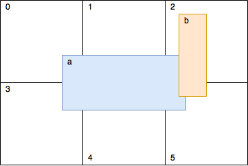
Function calculateCellsRanges() runs through each shape and calculates rows and columns in the grid where a shape resides.

Fill Grid

Each cell in the grid represented as a vector of shapes. If it’s empty during a frame the vector size will be zero. Obviously. In function fillGrid() we again run through all shapes and put them in corresponding cells (vectors). Later we’ll check shapes inside each cell for an intersection. But on the picture above we can see that the shapes a and b are both resides in cell 2 and 5. This means that we’ll check these two shapes twice. In order to fix this we need to add special code that will say - do we need to make a check. Knowing rows and columns of the grid for the shape makes this task trivial.

Solve Collisions

In my previous article we used the following algorithm for collision resolution - if objects were overlapped we moved them apart:

This added a lot of complexity - we had to recalculate bounding box every time we moved a shape. In order to reduce the number of recalculations, we added a special accumulator which accumulated all necessary position changes and later applied it to the shape only once. Anyway, we had to add mutexes for synchronization, the code was difficult to understand and wasn’t ready for use with FP.

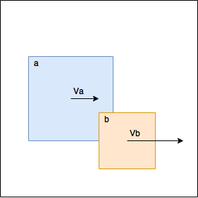
In the new attempt, we’ll not move objects to solve overlap at all. Moreover, we’ll make calculations only if it really necessary. On the picture, for example, there’s no need to solve collision - the shape b moves faster than the shape a and they moving apart from each other. Sooner or later they will stop to overlap by themselves - without our intervention. Of course, this is physically inaccurate, but if velocities and the simulation step are small then it looks ok. When the calculations are necessary we calculate velocity changes and store them together with the shape id.

Apply Velocities

Having velocity changes we pass them to the applyVelocities() function which just sums them up and applies to the shape. Again, there’s no physical meaning in this and probably there can be artifacts. But the purpose of this experiment was not a simulation correctness.

Result

After these simple steps, we have new data which is ready to be passed to the renderer. After rendering we’re repeating everything from the beginning again and again. Here’s a short video in order to prove that it works:

Conclusion

FP requires changing of thinking direction. But is it worth to do? Here’re my pros and cons:

Pros:

• Code readability. Together with SRP the code is easy to understand.
• Testability. Since the function’s result doesn’t depend on the environment and each function is a self-contained piece of code we have everything for testing.
• The most important point - the amazing ability for parallelization. Each function in our example can be called safely from any thread. Without synchronization primitives!

Cons:

• Performance. Recall that in previous article we could simulate 8000 shapes in one thread. Now we can do only 330.

When I worked in a game dev, trying to get the maximum of speed from each line of code, the approach we used today is not usable as it is. However, c++ is not a game dev only and I see a lot of places where FP can be applied.